RAMP on Predictive Maintenance for Aircraft Engines

Airlines seem to be successful businesses with strong management. Nonetheless, they literally bear high costs due to delays and cancellations that includes expenses on maintenance and compensations to travelers stuck in airports. Besides, they suffer from a non neglectable probability of failing on-flight accidents which can lead to disasters.
With nearly 30 percent of the total delay time caused by unplanned maintenance and at least 200 accident per year (including fatal accidents) , predictive analytics applied to fleet technical support is a reasonable solution. Predictive maintenance solutions are used to better manage data from aircraft health monitoring sensors. Knowing an aircraft’s current technical condition through alerts, notifications, and reports, employees can spot issues pointing at possible malfunction and replace parts proactively. Executives and team leads, in turn, can receive updates on maintenance operations, get data on tool and part inventory, and expenses via dashboards. With applied predictive maintenance, an airline can reduce expenses connected with expedited transportation of parts, overtime compensation for crews, and unplanned maintenance. If a technical problem did occur, maintenance teams could react to it faster with workflow organization software. The solution consists of analyzing data and metadata regarding detected maintenance activity. It helps engineers quickly evaluate a situation, for instance, to find out if this failure happened for the first time; if not, what can be done to fix it and how much time did it take to solve it previous times.
 |
Salma JERIDI, Aymen DABGHI, Aymen MTIBAA, Ahmed AKAKZIA
 |
1. Prognostics and Health Management
2. Business case
2.1 Introduction
2.2 Business Model
3. System and Damage Propoagation Modeling
3.1 System Modeling
3.2 Damage Propoagation Modeling
4. Data for the Challenge
5. Exploratory Data Analysis
6. Features Extraction
7. Classification model
8. Evaluation
9. Submitting to the online challenge
1. Prognostics and Health Management (PHM)
Prognostics and health management (PHM) is an engineering process of failure prevention and predicting reliability and remaining useful lifetime (RUL). It has become an important component of many engineering systems and products since it is very crucial to every industry to to detect anomalies, malfunctions and failures before they can damage the whole environment, including the system and the users, and may cause high costs for repairs on un-scheduled maintenance. Inspite of its main objective which is to ensure safety for users, it provides state of the heath of the components and systems which can create a scheduled list to program maintenance before damage. These maintenance tasks become therefore evidence-based scheduled There are two main categories of applications of PHM :
- Off-line PHM : It concerns systems where safety is not critical and the ratio of failures is very small.
- Real-time PHM : It concerns systems where safety is critical and that demand on-board monitoring capability.
There are two approaches that help define the health of a system as the extent of deviation or degradation from its expected typical operating performance which has to be determined accurately to prevent the failures : Data-driven and Model-driven. The former, as its name indicates, is based on data collection via real capturing or simulations based on theoretically-proved models. The latter is rather based on models that describe the system functionalities and specific knowledge.
 |
In this challenge, we would rather focus on the data-driven approach which uses monitored and historical data to learn the systems behaviours and perform prognostics. It is suitable for systems which are complex and with behaviours that cannot be assessed and deribed from first principles. It uses many algorithms that are quicker to implement and which are computationally more efficient to run compared with other techniques. The data is usually obtained via sensors. One problem of this approach is that the confidence level in the predictions depends on the available historical and empirical data. Besides, it requires some threshold values to be put by the operator which can sometimes be non-trivial.
Most efforts are focusing on data-driven approaches reflects the desire to harvest low-hanging fruit as compared to model-based approaches. Yet, it can be difficult to gain an access to statistically significant amounts of run-to-failure data and common metrics that allow a comparison between different approaches. Thus, a system model had been established in order to generate run-to failure data that can be utilized to develop, train and test prognostic algorithms. However, before entering into details of system modeling, let’s start by introducing the business case we will be considereing for this challenge.
2. Business Case :
2.1 Introduction :
Airlines seem to be successful businesses with strong management. Nonetheless, they literally bear high costs due to delays and cancellations that includes expenses on maintenance and compensations to travelers stuck in airports. Besides, they suffer from a non neglectable probability of failing on-flight accidents which can lead to disasters. With nearly 30 percent of the total delay time caused by unplanned maintenance and at least 200 accident per year (including fatal accidents) , predictive analytics applied to fleet technical support is a reasonable solution.
Predictive maintenance solutions are used to better manage data from aircraft health monitoring sensors. Knowing an aircraft’s current technical condition through alerts, notifications, and reports, employees can spot issues pointing at possible malfunction and replace parts proactively. Executives and team leads, in turn, can receive updates on maintenance operations, get data on tool and part inventory, and expenses via dashboards.
With applied predictive maintenance, an airline can reduce expenses connected with expedited transportation of parts, overtime compensation for crews, and unplanned maintenance. If a technical problem did occur, maintenance teams could react to it faster with workflow organization software. The solution consists of analyzing data and metadata regarding detected maintenance activity. It helps engineers quickly evaluate a situation, for instance, to find out if this failure happened for the first time; if not, what can be done to fix it and how much time did it take to solve it previous times.
Read further : https://www.forbes.com/sites/oliverwyman/2017/06/16/the-data-science-revolution-transforming-aviation/#6e2663227f6c
2.2 Business Model :
2.2.1 : Business Problem :
On the first hand, being ranked second after pilot error, aircraft’s system failure is still one of the five most common reasons for accidents. Equipment failures still account for around 20% of aircraft losses, despite improvements in design and manufacturing quality. While engines are significantly more reliable today than they were half a century ago, they still occasionally suffer catastrophic failures.
Sometimes, new technologies introduce new types of failure. In the 1950s, for example, the introduction of high-flying, pressurised jet aircraft introduced an entirely new hazard – metal fatigue brought on by the hull’s pressurisation cycle. Several high-profile disasters caused by this problem led to the withdrawal of the de Havilland Comet aircraft model, pending design changes.
On the other hand, if it is discovered that there is a maintenance issue with your aircraft, the flight will not embark until the issue has been fully addressed. Sometimes, these issues are being worked on even as passengers board the plane, meaning the delay the passenger experiences might take place entirely on the tarmac. Other times, in the case of larger issues, your airline might make the call to switch planes entirely for the safety of everyone involved. Thus, this would cost a lot of money for the airline company to handle.
On-flight accidents and delays cause enormous costs for the airlines each year. Therefore, this issue should be handled.
2.2.2: Our solution :
First, we have to understand two main concepts: airliners are complex mechanical wonders, and second, their maintenance and operation is very strictly and minutely regulated–and documented. This second point is essential to the aviation regulatory standard upheld by all major airlines, even though such detail must be correctly, diligently accomplished.
Our solution would be to use a data-driven approach in order to schedule the different maintenance tasks in advance. In consists of making use of the different sensors and telemetry available, which depend on the different conditions and modes to predict the order of priority for each engine. In this way, the client would be able to know which engines need to go through maintenance tasks immediately, and which can still wait.
Since we talked about the client, it can be an airline company trying to utilize historical data of equipment sensors to make data-driven decisions on its maintenance planning. Based on this analysis, the company will be able to estimate engine’s order of priority and optimize its maintenance operations accordingly.
2.2.3 : Predictive maintenance task :
As mentionned previously, reliably estimating remaining life holds the promise for considerable cost savings. In fact, that allows us to avoid unscheduled maintenance and to increase equipment usage, and unsures the operational safety improvements.
Some studies focus on predicting the Remaining Useful Life (RUL) of the engine of a part and its components, or the exact Time to Failure (TTF). For safety purpose, and considering the error of the predictive model, companies may define a safety threshold ie : a number of cycles that they add to the prediction made by the regressor. This fact makes the alternative of predicting if an asset will fail in different time windows relevant. We formulate then as a Multi-class classification problem and we define 4 four Time to Failure windows (4 classes) :
-
Class 0 : Very urgent maintenance : 0 to 10 cycles remaining before failure.
-
Class 1 : Aircraft maintenance periodic checks need to be deep and more detailed : 11 to 30 cycles remaining before failure.
-
Class 2 : Confident system : We can plan from this period the future maintenance date and provide the needed equipments : 31 to 100 cycles remaining before failure.
-
Class 3: Very confident system : Only periodic checks are needed : more than 101cycles remaining before failure.
We set the thresholds based on two key ideas of the predective maintenance : We want to predict the optimal time for maintenance by :
-
Minimizing the risk of unexpected failure.
-
Minimizing the cost of early and useless maintenance.
2.2.4 : Business metrics :
In our context, since the key aspect is to avoid failures, it is generally desirable to predict early as compared to predicting late. However, early predictions may also involve significant economic burden. We need then to choose a metric that heavely penalizes late predictions and takes of course into account the early prediction. To do so, we propose to combine two metrics :
Macro-averaged F1-score :
In this score, we need to define the weighted macro precision and recall score. We define the weights w.r.t to the previous condition. In fact,
- Assuming we have a One-vs-All (OvA) classifier, we calculate for each class (j) the corresponding precision and recall score :
- We average the performances of each individual class using a weight vector. In fact, making a late prediction for an engine having class 0 in the true labels is very dangerous. So, we need to avoid as much as possible the False Negative prediction for elements of the first class. The less is the true maintenance urgency, the more we can tolerate the FN rate. For this reason, we define the weighted Recall rate by :
- Similarly, falsely predicting that an aircraft is in class 3 is a late prediction and can cause damages specially if the true label is urgent maintenance. We can tolerate a bit more the case of class 2 because in some cases we can have an early prediction, but we still aim to penalize this kind of prediction. To do so, we define the weighted Precision as following :
- Finally, using the precision & recall calculated previoulsly, we define the macro-averaged F1-score by :
Multi-class logarithmic loss function :
We introduce the log loss function for our multicass problem :
\[LogLoss = − \frac{1}{N}\sum_i^N \sum_j^M y_{ij} \log(p_{ij}))\]where N is the number of instances, M is the number of different labels, $y_{ij}$ is the binary variable with the expected labels and $p_{ij}$ is the classificiation probability output by the classifier for the i-instance and the j-label.
Mixed score:
We define the final score function that we aim to minimize by :
\[L = LogLoss + (1 - F1_{score})\]3. System and Damage Propagation Modeling :
As mentionned in the introduction, data-driven prognostics faces the perennial challenge of the lack of run-to-failure data sets. In most cases realworld, it is time consuming and expensive to have such a data. In other cases, it’s is not even feasible. For example, an airlaine company cannot afford to wait for an engine failure in order to keep the failure exact date. Instead, they perform model/data driven maintenance to avoid the failures.
In order to face the lack of PHM data, a group of scientist in the U.S. National Aeronautics and Space Administration (NASA) worked on generating run-to-failure data that can then be utilized to develop, train, and test prognostic algorithms. In our challenge, we are going to use this generated data in order to train a robust model that can be used on real sensors data.
First, let’s introduce the two main concept of data generation.
3.1 System modeling
As the goal is to track and to predict the progression of damage in aircraft, the group of scienctist worked first on the simulation of a suitable system model that allows input variations of health related parameters and recording of the resulting output sensor measurements. To do so, they used C-MAPSS (Commercial Modular Aero Propulsion System Simulation) that allow the user to enter specific values of his/her own choice regarding operational profile, closed-loop controllers, environmental conditions, etc, and outputs a simulation of an engine model. A simplified diagram of engine simulated in C-MAPSS and a layout showing various modules and their connections as modeled in the simulation are shown in the following figures :
| Simplified diagram of engine simulated in C-MAPSS | Various modules and their connections as modeled in the simulation |
|---|---|
 |
 |
To simulate various degradation scenarios in any of the five rotating components of the simulated engine, C-MAPSS inputs the aircraft configuration. For example, to simulate HPC (High-Pressure Compressor) degradation, C-MAPSS requires the HPC flow and efficiency modifiers. The outputs include various sensor response surfaces. A total of 21 variables out of 58 different outputs available from the model were used in this challenge.
As an example of sensor response, we have :
- Total temperature at HPC outlet
- Total temperature at LPT outlet
- Pressure at fan inlet
- Total pressure in bypass-duct
- Total pressure at HPC outlet
- Physical fan speed
- Physical core speed, …
3.2 Damage propagation modeling
Having decided on the system model, the next step is to model the propagation of damage. The purpose here is to find a model-based method to generate the Time-to-failure (ttf) given the sensors data. In litterature, many degradation models have been proposed. As an example, The Arrhenius model has been used for a variety of failure mechanisms. The operative equation is: \(t_f = A * e^{\frac{\Delta H}{kT}}\)
With :
- $t_f$ is the time to failure,
- T is the temperature at the point when the failure process takes place,
- k is Boltzmann’s constant,
- A is a scaling factor, and
- $\Delta H$ is the activation energy.
In our case, For the purpose of a physics-inspired data-generation approach, we assume a generalized equation for wear which ignores micro-level processes but retains macro-level degradation characteristics. In addition to this propagation model, two important issues have been considered :
3.2.1 Initial Wear
Initial wear can occur due to manufacturing inefficiencies and are commonly observed in real systems. In the simulation, the degree of initial wear that an engine might experience with progressive usage was implemented following the calculations made by Chatterjee and Litt (see S. Chatterjee and J. Litt, “Online Model Parameter Estimation of Jet Engine Degradation for Autonomous Propulsion Control, “NASA, Technical Manual TM2003-212608, 2003. for more details)
3.2.2 Effects of between-flight maintenance
The effects of between-flight maintenance have not been explicitly modeled but have been incorporated as the process noise. Since there was no real data available to characterize true noise levels, simplistic normal noise distributions were assumed based on information available from the literature. Finally, To make the signal noise non-trivial, mixture distributions were used.
4. Data for the challenge
During this challenge, we are going to use the NASA’s public data set, result of Engine degradation simulation described previously. Four different sets were simulated under different combinations of operational conditions and fault modes (original data available here : https://ti.arc.nasa.gov/tech/dash/groups/pcoe/prognostic-data-repository/?fbclid=IwAR2ec11zAXo5KH5PcJO0axppSlajScvSrUL17xxbSqUiQ7YpVie31CCSw4s#turbofan)
For our case, we restrict our study to the combination of two data sets simulated under those conditions :
- Fault Modes : HPC and/or Fan module Degradation
- Simulation under sea level condition.
Data sets consists of multiple multivariate time series(unit of time is one cycle). Each data set is further divided into training and test subsets. Each time series is from a different engine, i.e, the data can be considered to be from a fleet of engines of the same type.
The engine is operating normally at the start of each time series, and develops a fault at some point during the series. In the training set, the fault grows in magnitude until system failure. In the test set, the time series ends some time prior to system failure. To conclude, the available data is the following :
- Training Data: The aircraft engine run-to-failure data.
- Test Data: The aircraft engine operating data without failure events recorded.
- Ground Truth Data: The true remaining cycles (True TTF) for each engine in the testing data.
In order to fit the data to the problem’s need, we brought the following modifications:
-
As the training data was not labeled and knowing the system failure cycle, we started by calculating the Time To Failure (TTF) of each observation and then we assigned them to the corresponding classes.
-
The true TTF available in the ground truth data correspond to the last observation of each engine(which is not its failure point). So in order to have more data for testing, we used these true TTF to generate the number of remaining cycles for the rest of the observations.
Import libraries
import pandas as pd
import numpy as np
import seaborn as sns
import matplotlib.pyplot as plt
from problem import get_train_data,  get_test_data

from sklearn.preprocessing import StandardScaler
from sklearn.metrics import confusion_matrix
from sklearn.metrics import accuracy_score , auc, classification_report, precision_score,recall_score,log_loss, roc_curve

from itertools import cycle
from sklearn.preprocessing import label_binarize
from scipy import interp
sns.set(font_scale=1.0)
Loading the data
We start by inspecting the training data
# Load train data
X_train , y_train = get_train_data()
X_train.shape , y_train.shape
((45351, 26), (45351,))
X_train.head()
| ID | Cycle | op_set_1 | op_set_2 | op_set_3 | s1 | s2 | ... | s15 | s16 | s17 | s18 | s19 | s20 | s21 | |
|---|---|---|---|---|---|---|---|---|---|---|---|---|---|---|---|
| 0 | 1 | 1 | -0.0007 | -0.0004 | 100.0 | 518.67 | 641.82 | ... | 8.4195 | 0.03 | 392 | 2388 | 100.0 | 39.06 | 23.4190 |
| 1 | 1 | 2 | 0.0019 | -0.0003 | 100.0 | 518.67 | 642.15 | ... | 8.4318 | 0.03 | 392 | 2388 | 100.0 | 39.00 | 23.4236 |
| 2 | 1 | 3 | -0.0043 | 0.0003 | 100.0 | 518.67 | 642.35 | ... | 8.4178 | 0.03 | 390 | 2388 | 100.0 | 38.95 | 23.3442 |
| 3 | 1 | 4 | 0.0007 | 0.0000 | 100.0 | 518.67 | 642.35 | ... | 8.3682 | 0.03 | 392 | 2388 | 100.0 | 38.88 | 23.3739 |
| 4 | 1 | 5 | -0.0019 | -0.0002 | 100.0 | 518.67 | 642.37 | ... | 8.4294 | 0.03 | 393 | 2388 | 100.0 | 38.90 | 23.4044 |
5 rows × 20 columns
The data consist of 45351 observations and 26 features. Each row is a snapshot of data taken during a single operational cycle, each column is a different variable. The columns correspond to:
-
1) Unit number or ID of the engine ( 200 unique IDs)
-
2) Time in cycles
-
3) to 5) Operational settings 1 to 3
-
6) to 26) Sensor measurements 1 to 21
These measurements include various sensor response surfaces and operability margins :
- s1 : Total temperature at fan inlet
- s2: Total temperature at LPC outlet
- s3 : Total temperature at HPC (High-Pressure Compressor) outlet
- s4: Total temperature at LPT outlet
- s5: Pressure at fan inlet
- s6 : Total pressure in bypass-duct
- s7 :Total pressure at HPC outlet
- s8: Physical fan speed
- s9 :Physical core speed
- s10: Engine pressure ratio (P50/P2)
- s11: Static pressure at HPC outlet
- s12: Ratio of fuel flow to Ps30
- s13: Corrected fan speed
- s14: Corrected core speed
- s15: Bypass Ratio
- s16: Burner fuel-air ratio
- s17: Bleed Enthalpy
- s18: Demanded fan speed
- s19: Demanded corrected fan speed
- s20: HPT coolant bleed
- s21: LPT coolant bleed
X_train.info()
<class 'pandas.core.frame.DataFrame'>
RangeIndex: 45351 entries, 0 to 45350
Data columns (total 26 columns):
ID          45351 non-null int64
Cycle       45351 non-null int64
op_set_1    45351 non-null float64
op_set_2    45351 non-null float64
op_set_3    45351 non-null float64
s1          45351 non-null float64
s2          45351 non-null float64
s3          45351 non-null float64
s4          45351 non-null float64
s5          45351 non-null float64
s6          45351 non-null float64
s7          45351 non-null float64
s8          45351 non-null float64
s9          45351 non-null float64
s10         45351 non-null float64
s11         45351 non-null float64
s12         45351 non-null float64
s13         45351 non-null float64
s14         45351 non-null float64
s15         45351 non-null float64
s16         45351 non-null float64
s17         45351 non-null int64
s18         45351 non-null int64
s19         45351 non-null float64
s20         45351 non-null float64
s21         45351 non-null float64
dtypes: float64(22), int64(4)
memory usage: 9.0 MB
$\rightarrow$ There is no missing values to deal with.
X_train.describe()
| ID | Cycle | op_set_1 | op_set_2 | op_set_3 | s1 | s2 | ... | s18 | s19 | s20 | s21 | |
|---|---|---|---|---|---|---|---|---|---|---|---|---|
| count | 45351 | 45351 | 45351 | 45351 | 45351.0 | 4.535100e+04 | 45351 | ... | 45351.0 | 45351.0 | 45351 | 45351 |
| mean | 104.447796 | 125.307049 | -0.000017 | 0.000004 | 100.0 | 5.186700e+02 | 642.559339 | ... | 2388.0 | 100.0 | 38.910178 | 23.346022 |
| std | 56.544862 | 87.813757 | 0.002191 | 0.000294 | 0.0 | 4.637337e-10 | 0.524596 | ... | 0.0 | 0.0 | 0.236600 | 0.141834 |
| min | 1 | 1 | -0.008700 | -0.000600 | 100.0 | 5.186700e+02 | 640.840000 | ... | 2388.0 | 100.0 | 38.140000 | 22.872600 |
| 25% | 57 | 57 | -0.001500 | -0.000200 | 100.0 | 5.186700e+02 | 642.180000 | ... | 2388.0 | 100.0 | 38.760000 | 23.254500 |
| 50% | 108 | 114 | 0 | 0 | 100.0 | 5.186700e+02 | 642.520000 | ... | 2388.0 | 100.0 | 38.900000 | 23.342400 |
| 75% | 152 | 174 | 0.001500 | 0.000300 | 100.0 | 5.186700e+02 | 642.900000 | ... | 2388.0 | 100.0 | 39.050000 | 23.430100 |
| max | 200 | 525 | 0.008700 | 0.000700 | 100.0 | 5.186700e+02 | 645.110000 | ... | 2388.0 | 100.0 | 39.850000 | 23.950500 |
8 rows × 17 columns
$\rightarrow$ The target labels consist of 4 classes representing Time to Failure windows.
# The target labels
y_train.unique()
array([3, 2, 1, 0])
5. Exploratory Data Analysis (EDA)
def dataCleaning(Data):

    """
    In order to have a proper visualisation,
    some pre-exploration of the data has been done
    leading to the following modifications
    """

    # Some features have all their values set to NaN in the correlation matrix, we simply drop them
    Data.drop(['s18', 's19','op_set_3'],axis=1, inplace=True)

    # Some feature have 0 correlation with target and the other features, we drop them too
    Data.drop(['op_set_1','op_set_2','s1','s5','s16'], axis=1,inplace=True)

    # Some features are highly correlated (>0.9), we drop one of them(s9,s14) (s8,s13)
    Data.drop(['s12','s13','s14'], axis=1,inplace=True)

    return Data
X_train = dataCleaning(X_train)
Distribution of all engines with regards to their failure cycles:
cycles_per_engine = pd.DataFrame(X_train.groupby('ID')['Cycle'].max())
cycles_per_engine.reset_index(level = 0 , inplace=True)
cycles_per_engine.columns = ['ID' , 'Cycles']
plt.figure(figsize=(12,6))
sns.distplot(cycles_per_engine.Cycles , bins= 10, kde=False)
plt.title("Distribution of engines with respect to their failure cycles")
Text(0.5, 1.0, 'Distribution of engines with respect to their failure cycles')
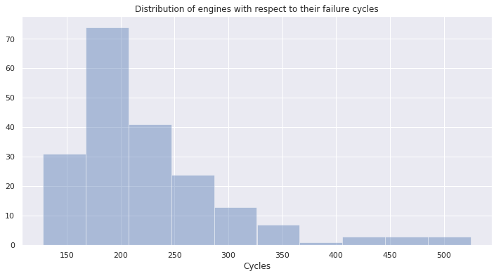
pd.DataFrame(cycles_per_engine.Cycles).quantile(0.75)
Cycles    256.25
Name: 0.75, dtype: float64
$\rightarrow$ We notice that : 75% of the engines fail before reaching 257 cycles.
# We will concatenat X_train and y_train for visualisation purposes.
y= pd.DataFrame(y_train)
X_conc= X_train
X_conc['labels']= y['labels'].values
Number of observations per class
ax= sns.countplot(x='labels', data=X_conc)
plt.title("Number of observation per class ")
Text(0.5, 1.0, 'Number of observation per class ')
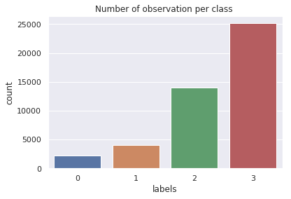
$\rightarrow$ We notice that : The distribution between classes seems to be imbalanced.
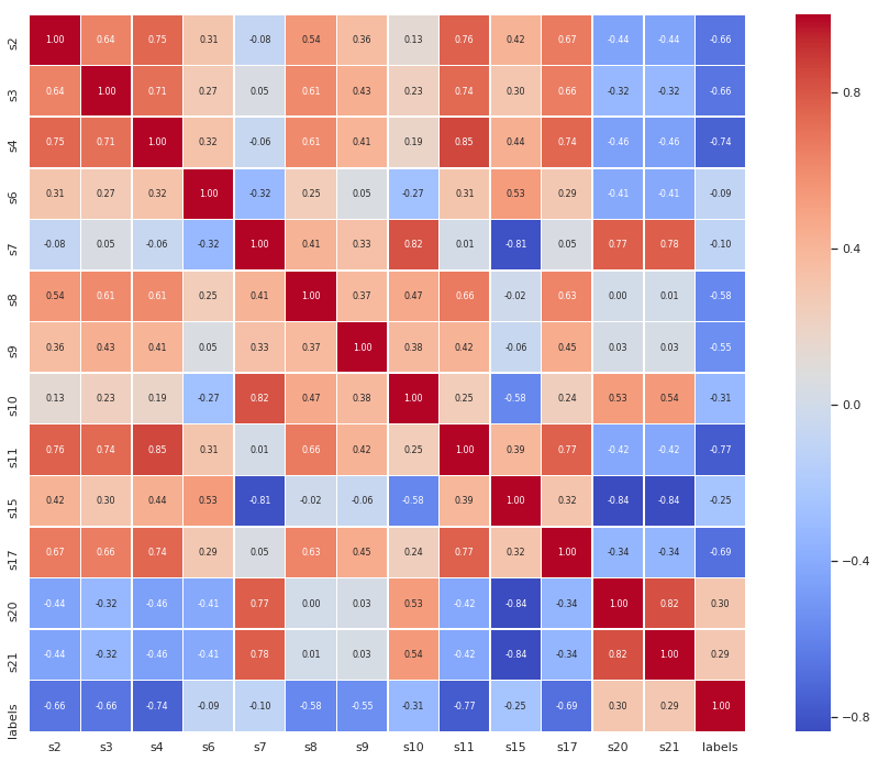
Feature correlation matrix :
feature_corr = X_conc.iloc[:,2:].corr()
plt.figure(figsize=(16,12))
sns.heatmap(feature_corr,annot=True,square=True,fmt='.2f',annot_kws={'size':8}, cmap='coolwarm',linewidths=.5)
plt.show()
Feature distributions :
ft_to_pairplot=['s2','s3','s4','s8','s9','s11','s17','labels']
g = sns.PairGrid(X_conc[ft_to_pairplot], hue="labels", vars=ft_to_pairplot[:-1])
g = g.map_diag(plt.hist, histtype="step", linewidth=3)
g.map_upper(plt.scatter)
g.map_lower(sns.kdeplot)
g = g.add_legend()
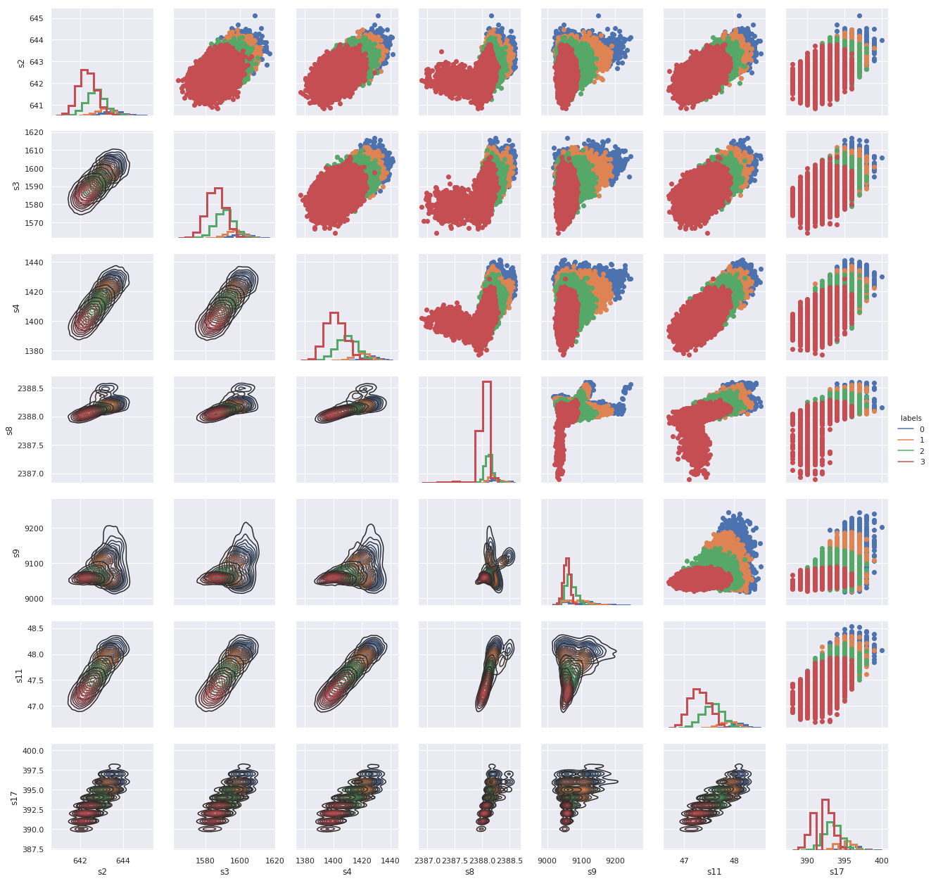
$\rightarrow$ Here we used a pairplot to see the bivariate relation between each pair of features and distribution of each feature. We notice that:
-
Classes are not seperated across all feature combinations, there is an overlap in their pairwise relationships.
-
Almost all features visualized above have normal distributions.
Relevant features inspection :
def viz_func(eng_id,df):

    """ Plot time series of a single engine.

        Args:
        eng_id (int64): The id of the engine considered.

    Returns:
        plots

    """
    subset=df[df.ID==eng_id]
    f = subset.Cycle.iloc[-1]
    fig, axes = plt.subplots(nrows=7, ncols=1, figsize=(12,14), sharex=True)

    print (" Features inspection for engine : "+str(eng_id))
    ## Tempreture at LPC :
    axes[0].plot(subset.Cycle , subset.s2)
    axes[0].legend(['s2(°R)'])
    axes[0].set_title('Tempretures at LPC outlet')

    ## Tempreture at HPC :
    axes[1].plot(subset.Cycle , subset.s3)
    axes[1].legend(['s3(°R)'])
    axes[1].set_title('Tempretures at HPC outlet')

    ## Tempreture at LPT :
    axes[2].plot(subset.Cycle , subset.s4)
    axes[2].legend(['s4(°R)'])
    axes[2].set_title('Tempretures at LPT outlet')

    ## Static pressure at HPC outlet

    axes[3].plot(subset.Cycle , subset.s11)
    axes[3].legend(['s11(psia)'])
    axes[3].set_title('Static pressure at HPC outlet')

    ## Physical core speed

    axes[4].plot(subset.Cycle , subset.s9)
    axes[4].legend(['s9(rpm)'])
    axes[4].set_title('Physical core speed')

    ## Physical fan speed

    axes[5].plot(subset.Cycle , subset.s8)
    axes[5].legend(['s8(rpm)'])
    axes[5].set_title('Physical fan speed')

    ## HPT coolant bleed
    axes[6].plot(subset.Cycle , subset.s20)
    axes[6].legend(['s20(lbm/s)'])
    axes[6].set_title('HPT coolant bleed')

    for ax in axes:
        ax.axvline(f-10,color='r',label='ttf =10')
        ax.axvline(f-30,color='g',label='ttf =30')
        ax.axvline(f-100,color='k',label='ttf =100')

    plt.legend(loc=6)
    print('**************')
    return fig , axes
Visualize randomly chosen engines :
Engines = X_conc['ID'].unique()
eng_ids = np.random.choice(Engines, size=3)
for eng in eng_ids:
    viz_func(eng,X_conc)
 Features inspection for engine : 54
**************
 Features inspection for engine : 90
**************
 Features inspection for engine : 6
**************
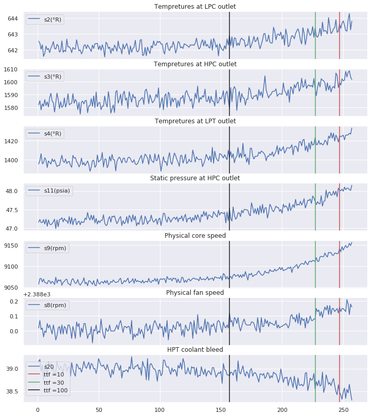
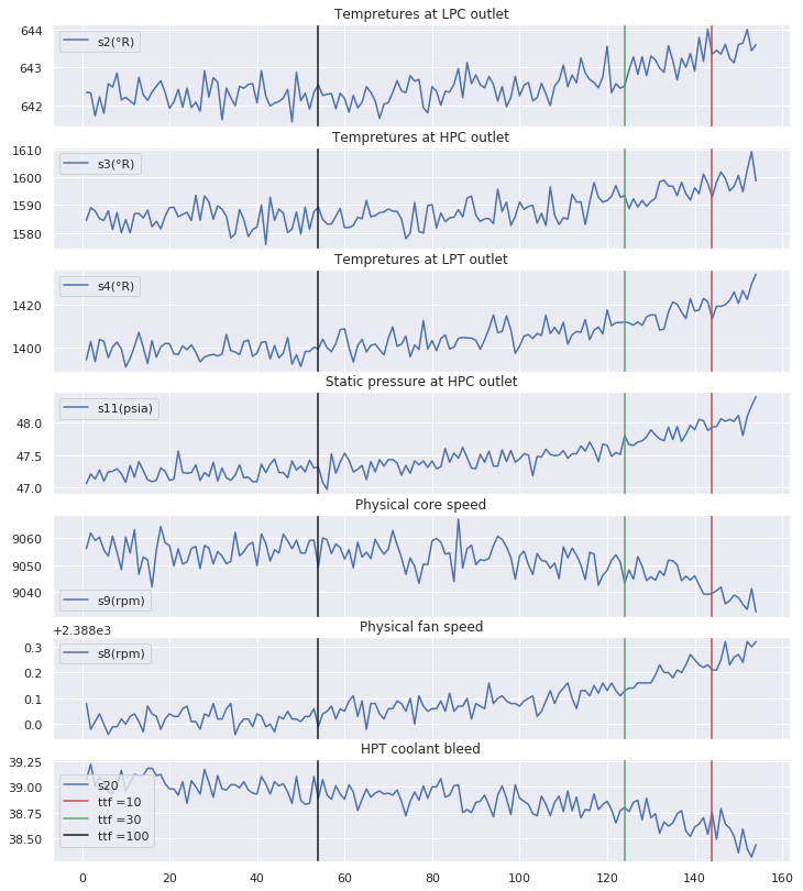
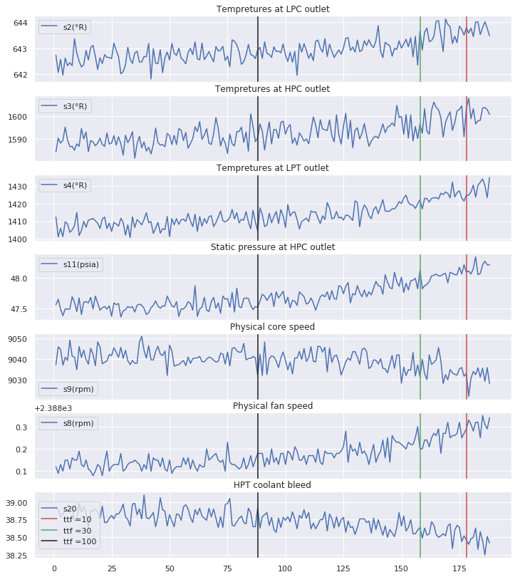
$\rightarrow$ It is clear that the behaviour of sensors measurements differ from one class to another and especially when the number of cycles gets close to the failure point. These sensors measurements should then have been more explored in order to extract other valuable and informative information.
Classes caracteristics:
sns.violinplot(data=X_conc,x="labels", y="s2")
<matplotlib.axes._subplots.AxesSubplot at 0x7fec555c0908>
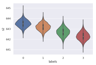
$\rightarrow$ Even though our features’ variances are quite low,these violinplots confirm the previous remark.
6. Features extraction
In order to have more informative and insightful data, we are going to generate new features using simple smoothing of the sensors’ measurements.
Since the observations related to each engine could be considered as time series independent from the other engines’ observations, the above functions will take that into consideration and apply rolling standard deviation (respectively mean) over a defined period of time (number of cycles) of a defined feature of a each engine seperately.
def rolling_std(data, feature, cycle_window, center=True):
    """
    For a given dataframe, compute the standard deviation over
    a defined period of time (number of cycles) of a defined feature

    Parameters
    ----------
    data : dataframe
    feature : str
        feature in the dataframe we wish to compute the rolling std from
    cycle_window : str
        string that defines the length of the cycle window passed to rolling
    center : bool
        boolean to indicate if the point of the dataframe considered is
        center or end of the window
    """

    df_to_return = pd.DataFrame()
    ids = data.ID.unique()
    name = '_'.join([feature, str(cycle_window), 'std'])
    for i in ids:
        sub_eng = data.loc[lambda df: df.ID == i, :]
        sub_eng.loc[:,name] = sub_eng[feature].rolling(cycle_window , center=center).std()
        sub_eng.loc[:,name] = sub_eng.loc[:,name].ffill().bfill()
        sub_eng.loc[:,name] = sub_eng[name].astype(sub_eng[feature].dtype)
        df_to_return = pd.concat([df_to_return , sub_eng], axis=0)
    return df_to_return
def rolling_mean(data, feature, cycle_window, center=False):
    """
    For a given dataframe, compute the mean over
    a defined period of time (number of cycles) of a defined feature

    Parameters
    ----------
    data : dataframe
    feature : str
        feature in the dataframe we wish to compute the rolling mean from
    cycle_window : str
        string that defines the length of the cycle window passed to rolling
    center : bool
        boolean to indicate if the point of the dataframe considered is
        center or end of the window
    """

    df_to_return = pd.DataFrame()
    ids = data.ID.unique()
    name = '_'.join([feature, str(cycle_window), 'mean'])
    for i in ids:
        sub_eng = data.loc[lambda df: df.ID == i, :]
        sub_eng.loc[:,name] = sub_eng[feature].rolling(cycle_window, win_type = 'hamming' , center=center).mean()
        sub_eng.loc[:,name] = sub_eng.loc[:,name].ffill().bfill()
        sub_eng.loc[:,name] = sub_eng[name].astype(sub_eng[feature].dtype)
        df_to_return = pd.concat([df_to_return , sub_eng], axis=0)
    return df_to_return
7. Classification model
In order to evaluate the performance of the submissions, we provide a test set that can be loaded similarly as follows:
X_test , y_test = get_test_data()
X_test.shape , y_test.shape
((29692, 26), (29692,))
X_test.head()
| ID | Cycle | op_set_1 | op_set_2 | op_set_3 | s1 | s2 | ... | s15 | s16 | s17 | s18 | s19 | s20 | s21 | |
|---|---|---|---|---|---|---|---|---|---|---|---|---|---|---|---|
| 0 | 1 | 1 | 0.0023 | 0.0003 | 100.0 | 518.67 | 643.02 | ... | 8.4052 | 0.03 | 392 | 2388 | 100.0 | 38.86 | 23.3735 |
| 1 | 1 | 2 | -0.0027 | -0.0003 | 100.0 | 518.67 | 641.71 | ... | 8.3803 | 0.03 | 393 | 2388 | 100.0 | 39.02 | 23.3916 |
| 2 | 1 | 3 | 0.0003 | 0.0001 | 100.0 | 518.67 | 642.46 | ... | 8.4441 | 0.03 | 393 | 2388 | 100.0 | 39.08 | 23.4166 |
| 3 | 1 | 4 | 0.0042 | 0.0000 | 100.0 | 518.67 | 642.44 | ... | 8.3917 | 0.03 | 391 | 2388 | 100.0 | 39.00 | 23.3737 |
| 4 | 1 | 5 | 0.0014 | 0.0000 | 100.0 | 518.67 | 642.51 | ... | 8.4031 | 0.03 | 390 | 2388 | 100.0 | 38.99 | 23.4130 |
5 rows × 20 columns
# Reload train data without modifications to test the feature extractor
X_train , y_train = get_train_data()
import sys
sys.path.insert(0, './submissions/starting_kit/')
from feature_extractor import FeatureExtractor
from classifier import Classifier
from sklearn.pipeline import make_pipeline

model = make_pipeline(FeatureExtractor(), Classifier())
model.fit(X_train, y_train)
y_pred = model.predict_proba(X_test)
y_pred_proba=y_pred
y_pred=np.argmax(y_pred,axis=1)
y_pred
array([3, 3, 3, ..., 2, 2, 2])
n_classes = 4
y_bin = label_binarize(y_test, classes=[0, 1, 2,3])
8. Evaluation
Sklearn metrics :
print ("Accuracy : ",accuracy_score(y_test, y_pred))
Accuracy : 0.8004176209079887
from sklearn.metrics import confusion_matrix
confusion_matrix(y_test,y_pred)
array([[    2,     0,    33,     0],
       [   20,     0,   533,    35],
       [    6,     0,  2728,  3144],
       [    0,     0,  2155, 21036]])
print(classification_report(y_test,y_pred))
              precision    recall  f1-score   support

           0       0.07      0.06      0.06        35
           1       0.00      0.00      0.00       588
           2       0.50      0.46      0.48      5878
           3       0.87      0.91      0.89     23191

   micro avg       0.80      0.80      0.80     29692
   macro avg       0.36      0.36      0.36     29692
weighted avg       0.78      0.80      0.79     29692
ROC curve
fpr = dict()
tpr = dict()
plt.figure(figsize=(10,8))
for i in range(4):
    fpr[i], tpr[i], _ = roc_curve(y_bin[:, i], y_pred_proba[:, i])


colors = cycle(['aqua', 'darkorange', 'cornflowerblue','r'])
for i, color in zip(range(n_classes), colors):
    plt.plot(fpr[i], tpr[i], color=color, lw=2,
             label='ROC curve of class {0} '
             ''.format(i))

plt.plot([0, 1], [0, 1], 'k--', lw=2)
plt.xlim([0.0, 1.0])
plt.ylim([0.0, 1.05])
plt.xlabel('False Positive Rate')
plt.ylabel('True Positive Rate')
plt.title('ROC-AUC curve for each class with sklearn metrics')
plt.legend()
plt.show()
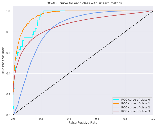
$\rightarrow$High accuracy does not mean a performant model, true and false positives should be taken into cosideration.The above results seem to be good but in reality the classes are imbalanced and have different order of importance (urgency). That’s why we defined our proper metrics that respond to the problem’s needs (weighted metrics).
Business metrics
def new_metrics(y_true,y_pred,y_pred_proba):
    ## Multiclass Logloss
    ll = log_loss(y_true, y_pred_proba)
    print("log_loss : ",ll)
    ## Weighted Precision
    weights = [0.1, 0.2, 0.3, 0.4]
    class_score = precision_score(y_true, y_pred, average=None)
    w_prec = np.sum(class_score * weights)
    print("Weighted Precision : ",w_prec)
    ## Weighted recall :
    weights_rec = [0.5, 0.3, 0.1, 0.1]
    class_score = recall_score(y_true, y_pred, average=None)
    w_rec = np.sum(class_score *weights_rec)
    print("Weighted recall : ",w_rec)
    ## Macro Average F1
    rec = w_rec
    prec = w_prec
    m_avg_f1= 2 * (prec * rec) / (prec + rec + 10 ** -15)
    print("Macro Average F1 : ",m_avg_f1)
    ## Mixed
    mixed = ll + (1 - m_avg_f1)
    print("Mixed : ",mixed)
new_metrics(y_test,y_pred,y_pred_proba)
log_loss :  0.5046380836599733
Weighted Precision :  0.5048226478263285
Weighted recall :  0.16568937431274927
Macro Average F1 :  0.24949216686796474
Mixed :  1.2551459167920087
def plot_classes_proba(eng_id , X_test , y_test , y_pred_proba):
    """ Plot the probability of a certain class for a single engine.

        Args:
        eng_id : The id of the engine considered.

    Returns:
        plots

    """
    # Generate a dataframe having the praobability of predicted classes, the engines IDs, the cycles
    # and the true classes

    df_y_pred_proba = pd.DataFrame(y_pred_proba , columns=['Class_0' , 'Class_1' , 'Class_2' , 'Class_3'])
    df_y_pred_proba['ID'] = X_test['ID'].copy()
    df_y_pred_proba['Cycle'] = X_test['Cycle'].copy()
    df_y_pred_proba['y_true'] = y_test


    subset = df_y_pred_proba[df_y_pred_proba.ID == eng_id]

    plt.figure(figsize=(12,8))

    plt.plot(subset.Cycle , subset.Class_0 , label='Class_0')
    plt.plot(subset.Cycle , subset.Class_1 , 'r' , label='Class_1')
    plt.plot(subset.Cycle , subset.Class_2 , 'g' , label='Class_2')
    plt.plot(subset.Cycle , subset.Class_3 , 'y' , label='Class_3')
    plt.legend()
    plt.title('Probability of class for engine : ' + str(eng_id))

    classes = subset.y_true.unique()

    c = 0
    clr = ['r','g','y']
    for i in range(len(classes)):
        t = subset[subset.y_true == classes[i]].shape[0]
        plt.axvline(c+t , color = clr[2-i])
        c = c + t

    return
eng_id = np.random.choice(Engines)
plot_classes_proba(eng_id , X_test , y_test , y_pred_proba)
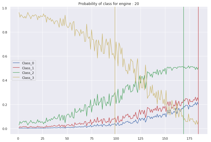
$\rightarrow$ In the figure above, we clearly notice that we have a problem of a late alarm. In fact, when the true value of the class is 1, our model assigns the higher probability to the class 2 (the segment between the red and green vertical lines). Therefore, we are predicting that our system is confident while it has in reality less than 30 cycles until failure. This can cause an unexpected damage to the aircraft’s engine.
$\rightarrow$ We can also be in the case of an early alarm. For example, an engine is a confident system while our model predicts it needs an urgent maintenance. This may involve a useless maintenance and a significant economic burden for the company.
9. Local testing
First install ramp-workflow, make sure that the python files feature_extractor.py and classifier.py are in the submission/starting_kit floder then run the following command.
!ramp_test_submission --submission starting_kit
[38;5;178m[1mTesting Predictive maintenance for aircraft engines[0m
[38;5;178m[1mReading train and test files from ./data ...[0m
[38;5;178m[1mReading cv ...[0m
[38;5;178m[1mTraining ./submissions/starting_kit ...[0m
[38;5;178m[1mCV fold 0[0m
/home/aymen/anaconda3/lib/python3.6/site-packages/sklearn/linear_model/logistic.py:758: ConvergenceWarning: lbfgs failed to converge. Increase the number of iterations.
"of iterations.", ConvergenceWarning)
/home/aymen/anaconda3/lib/python3.6/site-packages/sklearn/metrics/classification.py:1143: UndefinedMetricWarning: Precision is ill-defined and being set to 0.0 in labels with no predicted samples.
'precision', 'predicted', average, warn_for)
/home/aymen/anaconda3/lib/python3.6/site-packages/sklearn/metrics/classification.py:1143: UndefinedMetricWarning: Precision is ill-defined and being set to 0.0 in labels with no predicted samples.
'precision', 'predicted', average, warn_for)
[38;5;178m[1mscore mixed mc_ll w_prec w_rec[0m
[38;5;10m[1mtrain[0m [38;5;10m[1m1.13[0m [38;5;150m0.60[0m [38;5;150m0.67[0m [38;5;150m0.36[0m
[38;5;12m[1mvalid[0m [38;5;12m[1m1.15[0m [38;5;105m0.55[0m [38;5;105m0.63[0m [38;5;105m0.30[0m
[38;5;1m[1mtest[0m [38;5;1m[1m1.02[0m [38;5;218m0.41[0m [38;5;218m0.66[0m [38;5;218m0.27[0m
[38;5;178m[1mCV fold 1[0m
/home/aymen/anaconda3/lib/python3.6/site-packages/sklearn/linear_model/logistic.py:758: ConvergenceWarning: lbfgs failed to converge. Increase the number of iterations.
"of iterations.", ConvergenceWarning)
[38;5;178m[1mscore mixed mc_ll w_prec w_rec[0m
[38;5;10m[1mtrain[0m [38;5;10m[1m1.19[0m [38;5;150m0.60[0m [38;5;150m0.69[0m [38;5;150m0.29[0m
[38;5;12m[1mvalid[0m [38;5;12m[1m1.26[0m [38;5;105m0.65[0m [38;5;105m0.64[0m [38;5;105m0.28[0m
[38;5;1m[1mtest[0m [38;5;1m[1m1.09[0m [38;5;218m0.43[0m [38;5;218m0.64[0m [38;5;218m0.24[0m
[38;5;178m[1mCV fold 2[0m
/home/aymen/anaconda3/lib/python3.6/site-packages/sklearn/linear_model/logistic.py:758: ConvergenceWarning: lbfgs failed to converge. Increase the number of iterations.
"of iterations.", ConvergenceWarning)
[38;5;178m[1mscore mixed mc_ll w_prec w_rec[0m
[38;5;10m[1mtrain[0m [38;5;10m[1m1.25[0m [38;5;150m0.64[0m [38;5;150m0.62[0m [38;5;150m0.29[0m
[38;5;12m[1mvalid[0m [38;5;12m[1m1.21[0m [38;5;105m0.68[0m [38;5;105m0.64[0m [38;5;105m0.38[0m
[38;5;1m[1mtest[0m [38;5;1m[1m1.13[0m [38;5;218m0.47[0m [38;5;218m0.65[0m [38;5;218m0.23[0m
[38;5;178m[1mCV fold 3[0m
/home/aymen/anaconda3/lib/python3.6/site-packages/sklearn/linear_model/logistic.py:758: ConvergenceWarning: lbfgs failed to converge. Increase the number of iterations.
"of iterations.", ConvergenceWarning)
[38;5;178m[1mscore mixed mc_ll w_prec w_rec[0m
[38;5;10m[1mtrain[0m [38;5;10m[1m1.12[0m [38;5;150m0.60[0m [38;5;150m0.68[0m [38;5;150m0.37[0m
[38;5;12m[1mvalid[0m [38;5;12m[1m1.16[0m [38;5;105m0.61[0m [38;5;105m0.65[0m [38;5;105m0.34[0m
[38;5;1m[1mtest[0m [38;5;1m[1m1.05[0m [38;5;218m0.41[0m [38;5;218m0.64[0m [38;5;218m0.26[0m
[38;5;178m[1mCV fold 4[0m
/home/aymen/anaconda3/lib/python3.6/site-packages/sklearn/linear_model/logistic.py:758: ConvergenceWarning: lbfgs failed to converge. Increase the number of iterations.
"of iterations.", ConvergenceWarning)
[38;5;178m[1mscore mixed mc_ll w_prec w_rec[0m
[38;5;10m[1mtrain[0m [38;5;10m[1m1.10[0m [38;5;150m0.59[0m [38;5;150m0.68[0m [38;5;150m0.39[0m
[38;5;12m[1mvalid[0m [38;5;12m[1m1.22[0m [38;5;105m0.69[0m [38;5;105m0.65[0m [38;5;105m0.37[0m
[38;5;1m[1mtest[0m [38;5;1m[1m0.97[0m [38;5;218m0.43[0m [38;5;218m0.69[0m [38;5;218m0.34[0m
[38;5;178m[1m----------------------------[0m
[38;5;178m[1mMean CV scores[0m
[38;5;178m[1m----------------------------[0m
[38;5;178m[1mscore mixed mc_ll w_prec w_rec[0m
[38;5;10m[1mtrain[0m [38;5;10m[1m1.16[0m [38;5;150m[38;5;150m[38;5;150m[38;5;150m±[0m[0m[0m[0m [38;5;150m0.054[0m [38;5;150m0.61[0m [38;5;150m[38;5;150m[38;5;150m[38;5;150m±[0m[0m[0m[0m [38;5;150m0.018[0m [38;5;150m0.67[0m [38;5;150m[38;5;150m[38;5;150m[38;5;150m±[0m[0m[0m[0m [38;5;150m0.024[0m [38;5;150m0.34[0m [38;5;150m[38;5;150m[38;5;150m[38;5;150m±[0m[0m[0m[0m [38;5;150m0.041[0m
[38;5;12m[1mvalid[0m [38;5;12m[1m1.2[0m [38;5;105m[38;5;105m[38;5;105m[38;5;105m±[0m[0m[0m[0m [38;5;105m0.042[0m [38;5;105m[38;5;105m0.64[0m[0m [38;5;105m[38;5;105m[38;5;105m[38;5;105m±[0m[0m[0m[0m [38;5;105m0.051[0m [38;5;105m[38;5;105m0.64[0m[0m [38;5;105m[38;5;105m[38;5;105m[38;5;105m±[0m[0m[0m[0m [38;5;105m0.008[0m [38;5;105m0.33[0m [38;5;105m[38;5;105m[38;5;105m[38;5;105m±[0m[0m[0m[0m [38;5;105m0.038[0m
[38;5;1m[1mtest[0m [38;5;1m[1m1.05[0m [38;5;218m[38;5;218m[38;5;218m[38;5;218m±[0m[0m[0m[0m [38;5;218m0.054[0m [38;5;218m0.43[0m [38;5;218m[38;5;218m[38;5;218m[38;5;218m±[0m[0m[0m[0m [38;5;218m0.024[0m [38;5;218m0.66[0m [38;5;218m[38;5;218m[38;5;218m[38;5;218m±[0m[0m[0m[0m [38;5;218m0.016[0m [38;5;218m0.27[0m [38;5;218m[38;5;218m[38;5;218m[38;5;218m±[0m[0m[0m[0m [38;5;218m0.038[0m
[38;5;178m[1m----------------------------[0m
[38;5;178m[1mBagged scores[0m
[38;5;178m[1m----------------------------[0m
/home/aymen/anaconda3/lib/python3.6/site-packages/sklearn/metrics/classification.py:1143: UndefinedMetricWarning: Precision is ill-defined and being set to 0.0 in labels with no predicted samples.
'precision', 'predicted', average, warn_for)
[38;5;178m[1mscore mixed[0m
[38;5;12m[1mvalid[0m [38;5;12m[1m1.20[0m
[38;5;1m[1mtest[0m [38;5;1m[1m1.06[0m
Comments