Comparing Multi-task and Meta Reinforcement Learning

When tasks and goals are not known in advance, an agent may use either multitask learning or meta reinforcement learning to learn how to transfer knowledge from what it learned before. Recently, goal-conditioned policies and hindsight experience replay have become standard tools to address transfer between goals in the multitask learning setting. In this blog post, I show that these tools can also be imported into the meta reinforcement learning when one wants to address transfer between tasks and between goals at the same time. More importantly, I compare the computation gradients in MAML—a state of the art meta learning algorithm— to gradients in classic multi-task learning setups.

In an open-ended learning context [Doncieux et al. 2018], an agent faces a continuous stream of unforeseen tasks along its lifetime and must learn how to accomplish them. For doing so, two closely related reinforcement learning (RL) frameworks are available: multitask learning (MTL) and meta reinforcement learning (MRL).

Multitask learning was first defined in [Caruana 1997]. The general idea was to train a unique parametric policy to solve a finite set of tasks so that it would finally perform well on all these tasks. Various MTL frameworks have been defined since then [Yang and Hospedales 2014]. For instance, an MTL agent may learn several policies sharing only a subset of their parameters so that transfer learning can occur between these policies [Taylor and Stone 2009]. Multitask learning is the matter of an increasing research effort since the advent of powerful RL methods [Florensa et al. 2018; Veeriah et al. 2018; Ghosh et al. 2018].

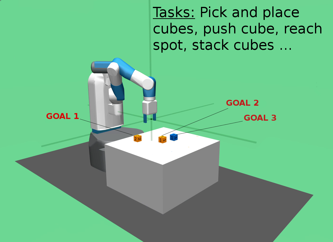
Fig.1 - The Fetch Environment with different tasks and goals.

But this effort came with a drift from the multitask to the multigoal context. Actually, the distinction between tasks and goals is not always clear. In this blog post, I will mainly rely on an intuitive notion illustrated in Figure 1 of task as some abstract activity such as push blocks or stack blocks, and we define a goal as some concrete state of the world that an agent may want to achieve given its current task, such as pick block “A” and place it inside this specific area. If we stick to these definition, a lot of work pretending to transfer between tasks actually transfer between goals. Anyways, for multigoal learning, goal-conditioned policies (GC-P) have emerged as a satisfactory framework to represent a set of policies to address various goals, as it naturally provides some generalization property between these goals. Besides, the use of Hindsight Experience Replay (HER) [Andrychowicz et al. 2017] has been shown to significantly speed up the process of learning to reach several goals when the reward is sparse. In this context, works trying to learn several tasks and several goals at the same time are just emerging (see Table 1 below).

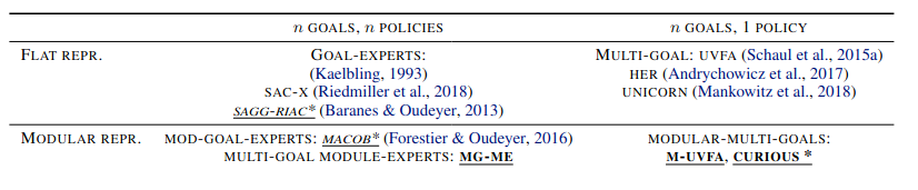
Table 1. Classification of multi-goal approaches (source [Colas et al. 2019]).

Meta reinforcement learning is a broader framework. Generally speaking, it consists in using inductive bias obtained from learning a set of policies, so that new policies for addressing similar unknown tasks can be learned in only a few gradient steps. In this latter process called fine tuning, policy parameters are tuned specifically to each new task [Rakelly et al. 2019]. The MRL framework encompasses several different perspectives [Weng 2019]. One consists in learning a recurrent neural network whose dynamics update the weights of a policy so as to mimic a reinforcement learning process [Duan et al. 2016; Wang et al. 2016]. This approach is classified as context-based meta-learning in [Rakelly et al. 2019] as the internal variables of the recurrent network can be seen as latent context variables. Another perspective is efficient parameter initialization [Finn et al. 2017], classified as gradient-based meta-learning. Here, we focus on a family of algorithms encompassing the second perspective which started with Model-Agnostic Meta-Learning MAML [Finn et al. 2017]. A crucial feature of this family of algorithms is that they introduce a specific mechanism to favor transfer between tasks, by looking for initial policy parameters that are close enough to the manifold of optimal policy parameters over all tasks.

Actually, though in principle MRL is more meant to address several tasks than several goals in the same tasks, in practice empirical studies often address the same benchmarks which are multigoal rather than multitask [Finn et al. 2017; Rothfuss et al. 2018; Rakelly et al. 2019]. Only a few papers truly transfer knowledge from one task to another [Zhao et al. 2017; Colas et al. 2019; Fournier et al. 2019], but at least the latter two do not classify themselves as performing MRL.

The common practice in MTL consists in sampling from all target tasks, which limits its applicability to the open-ended learning context, where some target tasks may not be known in advance. Besides, transfer between tasks in MTL, or rather between goals, usually relies on the generalization capability of the underlying function approximator, without any specific mechanism to improve it, resulting in potential brittleness when this approximator is not appropriate. Nevertheless, when applied to the multigoal setting using GCPs and HER, this approach has been shown to provide efficient transfer capabilities.

By contrast, in MRL, the test tasks are left apart during training. To ensure good transfer to these unseen tasks, the approach in MAML consists in iteratively refining the initial policy parameters so that a new task can be learned through only a few gradient steps. In principle, this latter transfer-oriented mechanism makes MRL more appropriate for open-ended learning, where the agent cannot train in advance on future unknown tasks.

In this part of the blog post, we compare the computation of gradients in MAML and the \mtl algorithm we used. At first glance, the differences are the following:

• MAML uses a meta-optimization step, making it necessary to distinguish gradient computation in the inner and outer update.

• MAML requires performing new rollouts after each update in order to obtain the validation trajectory set.

• In MAML, the meta-parameters only change at the end of each epoch. This means that back-propagation needs to be performed through the outer and the inner update. Hence, the gradients are always computed with respect to the initial parameters. By contrast, with MTL, the model parameters change at each update.

In the more detailed presentation given below, we are interested in the expression of the gradient at the end of a single epoch. Notations are provided bit by bit as we show the computational details.

MAML gradient

We initialize the model parameters \(\theta_0\) randomly. We sample a batch of \(N\) tasks and we perform \(k\) inner update for each task:

\[\begin{align*} \theta_0^i & = \theta_0\\ \theta_1^i & = \theta_0^i - \alpha \nabla_{\theta} \mathcal{L} (\theta_0^i, \mathcal{D}^{tr}_i)\\ \theta_2^i &= \theta_1^i - \alpha \nabla_{\theta} \mathcal{L} (\theta_1^i, \mathcal{D}^{tr}_i)\\ & ... \\ \theta_k^i &= \theta_{k-1}^i - \alpha \nabla_{\theta} \mathcal{L} (\theta_{k-1}^i, \mathcal{D}^{tr}_i)\\ \end{align*}\]

Where \(\mathcal{D}^{tr}_i\) corresponds to the trajectories obtained in the task \(i\) using the parameters before the considered update. At the end of the last inner update of the last task in the batch, we obtain a sequence of parameters {\(\theta_k^1, \theta_k^2, \theta_k^3, ..., \theta_k^N\)} for each of the \(N\) tasks. These parameters are used to generate new trajectories \(\mathcal{D}^{val}_i\) for each task \(i\).

In the outer loop, \maml uses the newly sampled trajectories to update the meta-objective:

\[\theta \leftarrow \theta - \beta g_{MAML},\]

where \(g_{MAML}\) is computed in [Wang et al. 2016]. Here we take back the same computations and add summation across all copies of task-specific parameters:

\[\begin{align*} g_{MAML} &= \nabla_{\theta} \sum_{i=1}^N \mathcal{L} (\theta_k^i, \mathcal{D}^{val}_i) \\ &= \sum_{i=1}^N \nabla_{\theta} \mathcal{L} (\theta_k^i, \mathcal{D}^{val}_i) \\ &= \sum_{i=1}^N \nabla_{\theta_k^i} \mathcal{L} (\theta_k^i, \mathcal{D}^{val}_i) . (\nabla_{\theta^i_{k-1}} \theta^i_k) ... (\nabla_{\theta^i_0} \theta^i_1) . (\nabla_{\theta} \theta^i_0)\\ &= \sum_{i=1}^N \nabla_{\theta_k^i} \mathcal{L} (\theta_k^i, \mathcal{D}^{val}_i) . {\displaystyle \prod_{j=1}^k \nabla_{\theta^i_{j-1}} \theta^i_j}\\ &= \sum_{i=1}^N \nabla_{\theta_k^i} \mathcal{L} (\theta_k^i, \mathcal{D}^{val}_i) . {\displaystyle \prod_{j=1}^k \nabla_{\theta^i_{j-1}} (\theta_{j-1}^i - \alpha \nabla_{\theta} \mathcal{L} (\theta_{j-1}^i, \mathcal{D}^{tr}_i))}\\ &= \sum_{i=1}^N \nabla_{\theta_k^i} \mathcal{L} (\theta_k^i, \mathcal{D}^{val}_i) . {\displaystyle \prod_{j=1}^k (I - \alpha \nabla_{\theta^i_{j-1}} (\nabla_{\theta} \mathcal{L} (\theta_{j-1}^i, \mathcal{D}^{tr}_i))}\\ \end{align*}\]

Multitask Learning algorithm gradient

In MTL, there is no distinction between an inner and an outer loop. The model parameters \(\theta_0\) are initialized randomly. In contrast to MAML, the gradients do not refer to the initial parameters but to the last updated one. We start by sampling a batch of \(N\) tasks. We perform \(k\) updates for each task sequentially:

\[\begin{align*} \theta_0^1 &= \theta_0 \\ \theta_1^1 &= \theta_0^1 - \alpha \nabla_{\theta_0^1} \mathcal{L} (\theta_0^1, \mathcal{D})\\ \theta_2^1 &= \theta_1^1 - \alpha \nabla_{\theta_1^1} \mathcal{L} (\theta_1^1, \mathcal{D})\\ & ... \\ \theta_k^1 &= \theta_{k-1}^1 - \alpha \nabla_{\theta_{k-1}^1} \mathcal{L} (\theta_{k-1}^1, \mathcal{D})\\ \theta_0^2 &= \theta_{k}^1 - \alpha \nabla_{\theta_{k}^1} \mathcal{L} (\theta_{k}^1, \mathcal{D})\\ & ... \\ & ... \\ \theta_{k-1}^N &= \theta_{k-2}^N - \alpha \nabla_{\theta_{k-2}^N} \mathcal{L} (\theta_{k-2}^N, \mathcal{D}),\\ \end{align*}\]

where \(\mathcal{D}\) is a shared set of trajectories between all tasks. Note that sharing the same buffer for different tasks comes with some constraints: tasks must share a common MDP structure, onlmy the reward is task-specific. This is the case of the \fetch robotics environments.

To get a mathematical expression of the \mtl gradient at the end of an epoch, which we note $g_{MTL}$, we use the recursive relation found above. For simplicity of notations, we note the sequence \((\theta_0^1, ..., \theta_k^1, \theta_0^2, ...\theta_{k-1}^2, ..., \theta_0^N, ..., \theta_{k-1}^N)\) = \((\psi_0, ..., \psi_{Nk})\):

\[\begin{align*} \psi_{Nk} &= \psi_{Nk-1} - \alpha \nabla_{\psi_{Nk-1}} \mathcal{L} (\psi_{Nk-1}, \mathcal{D})\\ &= \psi_{Nk-2} - \alpha \nabla_{\psi_{Nk-2}} \mathcal{L} (\psi_{Nk-2}, \mathcal{D}) - \alpha \nabla_{\psi_{Nk-1}} \mathcal{L} (\psi_{Nk-1}, \mathcal{D})\\ & ... \\ &= \psi_0 - \alpha \sum_{i=0}^{Nk-1} \nabla_{\psi_i} \mathcal{L} (\psi_i, \mathcal{D})\\ &= \psi_0 - \alpha g_{MTL}. \end{align*}\]

Since \(\psi_i = \theta^{i \div k + 1}_{i \% k}\), the overall update after on epoch is:

\[\theta \leftarrow \theta - \alpha g_{MTL}.\]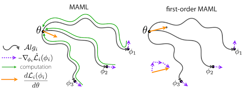

Fig.2-Diagram showing the path taken during the optimization step. $\mathcal{A}lg_i$ refers to the inner updates taken during task labeled $i$ (image taken from [Rajeswaran et al. 2019])

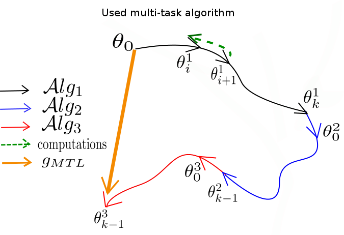
Fig.3-Diagram showing the path taken by the used multi-task algorithm. Here the computation is done at each step contrarily to what is shown in Fig 2, where computation is performed in the meta-update step. $\mathcal{A}lg_i$ refers to the updates taken during task labeled $i$.

Even though optimization-based \mrl and \mtl may seem very related, the gradients they compute are a lot different. The main differences are:

• During one single epoch, \mtl tends to update the model parameters during each gradient step, leading to more overall updates than optimization-based MRL. The latter tends to create copies of the meta-parameters, update each copy according to each task and then back-propagate through the inner optimization step to compute the gradients.

• Back-propagating through the inner optimization-step leads to second-order gradients derivative computations. The considered loss functions are differentiable almost everywhere. Computing the second-order derivative may be tricky. In fact, back-propagating through the inner-updates may lead to unstable gradients.

\[\begin{align*} \boxed{ \begin{array}{rcl} g_{MAML} & = & \sum_{i=1}^N \nabla_{\theta_k^i} \mathcal{L} (\theta_k^i, \mathcal{D}^{val}_i) . {\displaystyle \prod_{j=1}^k (I - \alpha \nabla_{\theta^i_{j-1}} (\nabla_{\theta} \mathcal{L} (\theta_{j-1}^i, \mathcal{D}^{tr}_i))} \\ g_{MTL} & = & \sum_{i=0}^{Nk-1} \nabla_{\psi_i} \mathcal{L} (\psi_i, \mathcal{D}) \end{array} } \end{align*}\]

1. Doncieux, S., Filliat, D., Dı́az-Rodrı́guez Natalia, et al. 2018. Open-ended Learning: a Conceptual Framework based on Representational Redescription. Frontiers in Robotics and AI 12.
2. Caruana, R. 1997. Multitask Learning. Machine Learning 28, 1, 41–75.
3. Yang, Y. and Hospedales, T.M. 2014. A unified perspective on multi-domain and multi-task learning. arXiv preprint arXiv:1412.7489.
4. Taylor, M.E. and Stone, P. 2009. Transfer learning for reinforcement learning domains: A survey. Journal of Machine Learning Research 10, Jul, 1633–1685.
5. Florensa, C., Held, D., Geng, X., and Abbeel, P. 2018. Automatic Goal Generation for Reinforcement Learning Agents. International Conference on Machine Learning, 1514–1523.
6. Veeriah, V., Oh, J., and Singh, S. 2018. Many-Goals Reinforcement Learning. arXiv preprint arXiv:1806.09605.
7. Ghosh, D., Gupta, A., and Levine, S. 2018. Learning Actionable Representations with Goal-Conditioned Policies. arXiv preprint arXiv:1811.07819.
8. Andrychowicz, M., Wolski, F., Ray, A., et al. 2017. Hindsight Experience Replay. arXiv preprint arXiv:1707.01495.
9. Colas, C., Oudeyer, P.-Y., Sigaud, O., Fournier, P., and Chetouani, M. 2019. CURIOUS: Intrinsically Motivated Multi-Task, Multi-Goal Reinforcement Learning. International Conference on Machine Learning (ICML), 1331–1340.
10. Rakelly, K., Zhou, A., Quillen, D., Finn, C., and Levine, S. 2019. Efficient off-policy meta-reinforcement learning via probabilistic context variables. arXiv preprint arXiv:1903.08254.
11. Weng, L. 2019. Meta Reinforcement Learning. lilianweng.github.io/lil-log.
12. Duan, Y., Schulman, J., Chen, X., Bartlett, P.L., Sutskever, I., and Abbeel, P. 2016. RL^2: Fast reinforcement learning via slow reinforcement learning. arXiv preprint arXiv:1611.02779.
13. Wang, J.X., Kurth-Nelson, Z., Tirumala, D., et al. 2016. Learning to reinforcement learn. arXiv preprint arXiv:1611.05763.
14. Finn, C., Abbeel, P., and Levine, S. 2017. Model-agnostic meta-learning for fast adaptation of deep networks. Proceedings of the 34th International Conference on Machine Learning-Volume 70, JMLR. org, 1126–1135.
15. Rothfuss, J., Lee, D., Clavera, I., Asfour, T., and Abbeel, P. 2018. Promp: Proximal meta-policy search. arXiv preprint arXiv:1810.06784.
16. Zhao, C., Hospedales, T., Stulp, F., and Sigaud, O. 2017. Tensor-based knowledge transfer across skill categories for robot control. Proceedings IJCAI.
17. Fournier, P., Sigaud, O., Chetouani, M., and Colas, C. 2019. CLIC: Curriculum Learning and Imitation for feature Control in non-rewarding environments. arXiv preprint arXiv:1901.09720.
18. Rajeswaran, A., Finn, C., Kakade, S., and Levine, S. 2019. Meta-Learning with Implicit Gradients. arXiv preprint arXiv:1909.04630.